A sonorant detection scheme using Mel-frequency cepstral coefficients and support vector machines (SVMs) is presented and tested in a variety of noise conditions. Adapting the classifier threshold using an estimate of the noise level is used to bias the classifier to effectively compensate for mismatched training and testing conditions. The adaptive threshold classifier achieves low frame error rates using only clean training data without requiring specifically designed features or learning algorithms.

The frame-by-frame SVM output is analyzed over longer time periods to uncover temporal modulations related to syllable structure which may aid in landmark-based speech recognition and speech detection. Appropriate filtering of this signal leads to a representation which is stable over a wide range of noise conditions. Using the smoothed output for landmark detection results in a high precision rate, enabling confident pruning of the search-space used by landmark-based speech recognizers.

Introduction

There has recently been considerable research undertaken to move automatic speech recognition systems away from the dominant frame-based HMM models to ones which utilize a segment-based or landmark-based approach [1,2,3]. Such methods require finding perceptually important points within the speech signal, referred to as landmarks. Landmarks may correspond to boundaries of phonetic segments (e.g. at a vowel-fricative transition), or they may occur near the center of a phonetic segment (e.g. the point of maximal energy in a vowel). A key step in implementing such a system is to reliably determine the location of these landmarks regardless of the acoustic environment.

It is likely that some types of landmarks will be inherently easier to detect in adverse conditions. Such landmarks could provide "islands of reliability" from which recognition of the utterance could be centered around. Even a very small number of reliable landmarks can significantly reduce the search space of possible segmentations when decoding an utterance.

One feature which may provide landmarks that can be robustly estimated is that of +sonorant. In noisy speech, the syllabic nuclei tend to be one of the last cues to be heard through the noise. Determining the location of peaks in sonority would provide a reliable basis for recognition as well as aiding in the detection of speech in heavy noise.

Related Work

Feature-based landmark detection has received considerable attention in recent years. Systems for discovering feature-based landmarks have been proposed [4,5], how one might use landmarks for lexical access has been investigated [1], and full recognition systems have been tested [3]. However, there has been less concentration on testing such systems in the presence of noise.

The problem of frame-based sonorant detection in noise has been investigated in [6], in which a novel statistical model is designed to combine features extracted from multiple frequency bands. Their model is shown to out-perform a classifier based on cepstra and Gaussian mixture models, and achieves low frame error rates in a variety of noise conditions. The setup of this experiment is done in a way to compare to these results.

Frame-based Sonorant Detection

While our ultimate goal is to detect locations of landmarks, we begin with a frame-based sonorant binary classifier. To ensure reliable phonetic-level transcriptions, the TIMIT corpus [7] is used for all experiments. For each utterance, 14 Mel-frequency cepstral coefficients (MFCCs) are computed every 10 ms over a 25.6 ms hamming window, with cepstral means subtracted over 500 ms. TIMIT trascriptions are used to label each frame +sonorant for vowels, semi-vowel and nasals, and -sonorant for fricitives, stops, and non-speech. All frames are placed into one of the two categories. To compare with other studies [6], 380 random sx and si TIMIT utterances were selected for training, and 110 for testing. Noisy speech is simulated by adding noise samples from the NOISEX database [8].

Binary classification is performed on each 14 element vector using a support vector machine (SVM). (All experiments used the SVMLight software package [9]). SVMs are well suited for binary classification tasks, have a strong theoretical foundation, and have shown considerable success in a variety of domains. Experiments were done with a linear kernel and a radial-basis function (RBF) kernel of the form K(x,y)=exp(-γ||x-y||^2). The width parameter γ=1e-7 was chosen by cross validation and used throughout this paper.

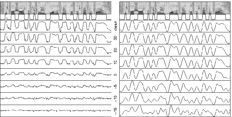
The frame-by-frame SVM outputs for a sample test utterance are shown on the left side of Figure 1. The SVM used for this example used a linear kernel and was trained on only clean speech. To calculate frame error rates from these outputs, a threshold must be chosen.

Figure 1: Spectrogram of an example test utterance with its ideal sonorant frame labels derived from TIMIT transcriptions. The panels on the left show SVM outputs at various levels of white noise. The vertical axes are the same in each case. The right side shows these outputs smoothed and scaled as described in Section 4.

SVM Threshold Adaptation

The linear SVM constructs a hyperplane in the dimension of the input vectors which best separates the two classes (in some sense). The resulting decision rule for the classification of frame i, represented by the feature vector xi is given by,

In the standard formulation the threshold λ is set to zero so that the decision rule simply corresponds to determining which side of the separating hyperplane (defined by w_0 and b_0) the vector x_i is located.

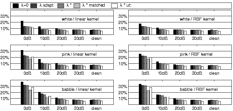
However, after we have set w_0 and b_0 in training, we can change the value of λ to bias a particular class. Figure 2 shows several examples of how choosing λ optimally can affect the overall error rate. λ* denotes the optimal threshold (in the sense it minimizes total error) if a single λ is chosen for each noise condition (level and type), while λ* utt represents choosing an optimal threshold for each testing utterance. All results shown here are trained only on clean speech, except λ* matched, which is trained on each condition separately (both noise type and level). Although not shown in the figure, tests indicated that when training and test conditions are matched, λ*=0.

Figure 2: Frame classification error results in different noise conditions using two different SVM kernels. All bars except λ* matched are trained on clean speech and use different thresholds to compute error rate.

These results show that λ=0 becomes further from the optimal threshold choice as the level of noise increases (i.e. as the amount of mismatch between training and testing data increases). Therefore, frame error rate may be reduced by a better choice of the threshold. Because most noise sources will more closely resemble -sonorant, than +sonorant sounds, the classifier will most likely bias all outputs toward -sonorant as the noise level increases. Therefore, adjusting λ based on an SNR estimate may be a reasonable way to attempt to compensate for this bias.

Estimating Optimal Threshold with SNR Estimate

Signal-to-noise ratio estimation is done by constructing a histogram of frame energies for each utterance. For stationary noise, the frames consisting of noise only (pauses in the speech) will accumulate, and a peak in the histogram will occur at the power level of the noise. Frames consisting of speech plus noise will contribute to a wider portion of the histogram, but will often produce a peak which can give an estimate of the speech power level (or the level of speech plus noise). The difference between the two major peaks will give not the SNR value itself, but some measure that is a good indicator of SNR (similar to the posterior signal-to-noise ratio [10].

Viewing frame histograms of a large number of utterances will have clearly defined peaks. Histograms of frames from a single utterance will not have such a well-defined shape, so simple peak-picking is unreliable. Therefore, to find the two modes, the Expectation Maximization (EM) algorithm was used to model the histogram as the sum of two Gaussian distributions. The difference in peaks was taken to be the difference between the means of the two distributions.

For each training utterance, the SNR measure was computed and the (utterance-level) optimal threshold was calculated for each trained SVM. During testing, first the SNR measure is calculated on the test utterance. K-nearest neighbors (k=10) is then used on the training data to map an SNR measure to the threshold, λ.

Frame-based Results

Adapting the threshold for each utterance as described leads the results given by λ adapt shown in Figure 2. The adaptive threshold gives considerable performance gains over keeping a zero threshold as the noise level increases, particularly for the linear kernel. Theλ adapt plot is very close to the λ* (optimal over noise condition) plot in all cases, which indicates that the SNR estimation technique was successful. For white noise, λ adapt gives performance on clean training data near to that of λ* matched. From equation (1), it is clear that adjusting λ is equivalent to keeping a zero threshold and adjusting b_0. So, it is somewhat surprising that a change in the single parameter b_0 can give equal performance to re-optimizing all parameters with matched data.

In comparing kernels, the RBF kernel outperforms the linear kernel at low SNR when both are using λ=0. However, when using the described threshold adaptation, the two kernels have very similar performance. Overall, these results are comparable to the sonorant detector of [6], without using a specifically designed learning algorithm and requiring only the ``off-the-shelf'' signal representation of MFCCs.

Landmark Detection

While frame-error rate is a good measure to compare classifiers, the ultimate goal is the ability to reliably detect the landmarks corresponding to peaks in sonority. To attempt this, we exploit the characteristic pattern of sonorant/non-sonorant regions which roughly correspond to the pattern of syllables. This pattern may be a key to not only robustly determining the sonorant landmarks, but also determining the presence of speech in heavy noise conditions.

In the 380 training utterances, sonorant landmarks (here defined as the midpoint of any continuous +sonorant frames) are spaced apart according to the distribution shown in Figure 3. This figure shows that very few sonorant landmarks are separated by less than 100 ms, and that modulations of sonorant levels generally occur in the range 2-10 Hz (100-500 ms). Other studies have shown that processing to concentrate on syllable-rate modulations can lead to noise robust representations [11]. Therefore, filtering to isolate this range of frequencies may help uncover landmark locations.

Figure 3: Histogram showing the distribution of time between sonorant landmarks in the training set.

Results

The SVM outputs are smoothed with an 11th order low-pass butterworth filter with cutoff frequency of 10 Hz, then shifted and scaled to occupy the range [-1,1]. The right side of Figure 1 shows the results of processing the original outputs. This measurement appears quite robust. The overall shape is fairly constant down to 0 dB and below, and the locations of the major peaks remain stable. This is similar to recent work in which similar processing (smoothing, scaling, and shifting) was performed on features for ASR, resulting in improved performance in noise [12].

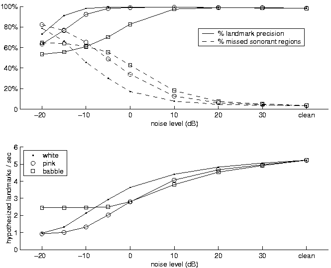
Figure 4 displays some quantitative results of landmark detection by choosing peaks in the filtered SVM output. Several heuristics are used to prune spurious and low peaks. These results have the general characteristics desired: as the noise level increases, the system may not be able to pinpoint as many landmarks (i.e. the number of hypothesized landmarks decreases), but it maintains a high precision for those that it does select. While the white and pink noise conditions give good results, the babble condition is considerably worse (performance on babble is approximately that of white at 20 dB lower SNR). This is to be expected since babble noise may actually contain sonorant segments, which would require higher-level mechanisms to distinguish background and foreground.

Figure 4: Landmark detection results using linear SVM trained on clean speech. Precision is the percentage of hypothesized landmarks falling within sonorant regions. A missed sonorant region is one with no hypothesized landmarks.

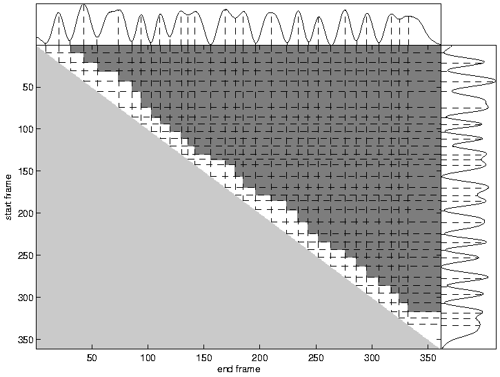
Figure 5: Example of pruning the segment search space using landmark detection. Each point in the upper triangle represents a candidate segment. The dark gray area is eliminated by not allowing any segments to span two sonorant landmarks (peaks or troughs).

Applications and Discussion

For 99.8% of the 6300 TIMIT utterances considered, the end of the utterance occurs within 400 ms of the end of the last sonorant frame. All 6300 utterances begin within 300 ms prior to the beginning of the first sonorant frame. Therefore, a reliable sonorant detector could be the basis for a robust speech end-pointer. It is likely that in heavy noise conditions, a detector based on sonorant detection could be more robust than either simple energy-based end-pointers, or classifiers trained on discriminating speech and non-speech.

The repetition of sonorant/non-sonorant regions in speech results in the classifier output showing a pattern roughly corresponding to a pattern of syllables which is likely very characteristic of typical speech. Recent work has shown that exploiting temporal modulations on the order of the syllable rate can lead to robust speech/non-speech classification of audio databases [13]. One technique for such a classifier would be a frame-based sonorant detector, followed by a binary classifier trained to detect syllable-like modulations in the smoothed output.

An application that can benefit from a robust landmark detector is segment-based speech recognition. In the SUMMIT speech recognition system [2], decoding consists of a search through possible segmentations of an utterance. Pruning of this segmentation-space before decoding can lead to in improvements in both speed and accuracy. Figure 5 shows one way to visualize all possible segments for a single utterance. Each point in the upper triangle represents a possible segment. While there are many ways to use feature detectors to either eliminate or select segments, this example shows the results from not allowing any segment to span either two peaks or two troughs in the smoothed sonorant detection output. Using this simple method on the entire test set eliminates over 85% of the segments to consider while discarding less than 4% of the true phonetic segments for all white noise conditions down to -15 dB SNR.

Conclusion

An SVM trained on MFCCs extracted from clean speech can classify frames as +sonorant and -sonorant at various noise levels with a low error rate. An SNR estimate can be reliably used to bias the classifier to account for some of the variation between training and testing conditions. Processing the SVM outputs to locate syllable-like modulations can lead to robust detection of landmarks corresponding to peaks in sonority. In extreme noise conditions such landmarks may offer some "islands of reliability" around which further exploration of the signal can be based.

References:

[1] Stevens, K. N. "Toward a model for lexical access based on acoustic landmarks and distinctive features," J. Acoust. Soc. Am., April 2002.

[2] J. Glass. "A Probabilistic Framework for Segment-Based Speech Recognition," Computer Speech and Language vol. 17, pp. 137-152, 2003.

[3] M. Hasegawa-Johnson et. al, "Landmark-Based Speech Recognition: Report of the 2004 Johns Hopkins Summer Workshop," in ICASSP, 2005.

[4] A. Juneja and C. Espy-Wilson, "Speech Segmentation Using Probabilistic Phonetic Feature Hierarchy and Support Vector Machines," in IJCNN 2003.

[5] P. Niyogi and C. Burges and P. Ramesh, "Distinctive Feature Detection Using Support Vector Machines," in ICASSP, 1998.

[6] L. K. Saul and M. G. Rahim and J. B. Allen, "A statistical model for robust integration of narrowband cues in speech," Computer Speech and Language, vol. 15, pp. 175-194, 2001.

[7] L. Lamel and R. Kassel and S. Seneff, "Speech database development: Design and analysis of the acoustic-phonetic corpus," in DARPA Speech Recognition Workshop, 1986.

[8] A. Varga and H. J. M. Steeneken and M. Tomlinson and D. Jones, "The Noisex-92 Study on the Effect of Additive Noise on Automatic Speech Recognition," Technical Report, DRA Speech Research Unit.

[9] T. Joachims, "SVMLight," http://svmlight.joachims.org.

[10] A. Surendran and S. Sukittanon and J. Platt, "Logistic Discriminative Speech Detectors using Posterior SNR," in ICASSP, 2004.

[11] S. Greenberg and B.Kingsbury, "The Modulation Spectrogram: In Pursuit of and Invariant Representation of Speech," in ICASSP 1997.

[12] C.-P. Chen and J. Bilmes and D. Ellis, "Speech Feature Smoothing For Robust ASR," in ICASSP 2005.

[13] M. Mesgarani and S. Shamma and M. Slaney, "Speech Discrimination Based on Multiscale Spectro-temporal Modulations," in ICASSP 2004.