|
Word Acquisition Using Unsupervised
Acoustic Pattern Discovery
Alex S. Park & James R. Glass
Introduction
We are working on a conceptually simple algorithm which can analyze an
audio recording and automatically discover and identify recurring patterns
which are likely to be significant with respect to the content of the
recording. The initial component of our algorithm is a completely unsupervised
method for grouping acoustically similar patterns into clusters using
pair-wise comparisons. Unlike traditional approaches to speech processing
which use an automatic speech recognizer, this clustering process does
not utilize a pre-specified lexicon. There are many ways in which the
clusters can be used: for directly summarizing unprocessed audio streams,
for initializing a lexicon prior to performing more exhaustive recognition,
or for performing information retrieval tasks on the recording. In [1],
we first introduced and demonstrated the utility of our pattern discovery
method for augmenting audio information retrieval. Here, we discuss extensions
to our original approach which allow us to use the clusters to automatically
identify words in the audio stream without explicitly relying on an ASR
system.
Approach
Our approach can be summarized in 3 main stages which are listed and
described below.
- Segmental Dynamic Time Warping
Typically, dynamic time warping (DTW) is used to find the optimal
global alignment between two whole word exemplars. In our work, we
face the problem of aligning two continuous speech utterances together
to find matching regions that correspond to common words or phrases.
This type of scenario requires that we find local alignments of matching
subsequences rather than the single globally optimal
alignments.
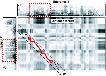
In order to address these limitations, we introduced a segmental
variation of DTW in [1] which is illustrated in
Figure 1. After computing the distance matrix betwen two utterances,
constrained diagonal bands of width W are searched for alignment
paths. The constrained bands serve two purposes: First, via the width
parameter W, they limit the amount of temporal distortion
that can occur between two sub-utterances during alignment. Second,
they allow for multiple alignments, as each band corresponds to another
potential path with different start and end points from the global
alignment path.
In practice, we use silence detection to break the audio stream into
separate utterances and then repeat the segmental DTW process for
each pair of utterances. As utterances are compared against each other,
the concentration of path fragments at particular locations in the
audio stream will indicate higher recurrence of the pattern occuring
at that location.
|
| Figure 1: The segmental DTW algorithm.
As in normal DTW, the distance matrix is computed between
two utterances. The matrix is then cut into overlapping diagonals
(only one shown here) with width W. The optimal alignment
path within each diagonal band is then found using DTW and
the resulting path is trimmed to the least average subsequence.
Finally, the trimmed alignment paths are retained as the subsequence
alignments between |
- Node Extraction
The result of the segmental DTW phase is a set of alignment paths
distributed throughout the audio stream. Although the alignment paths
overlap common time regions, path boundaries typically do not coincide
with each other and multiple intervals exist for each point in time.
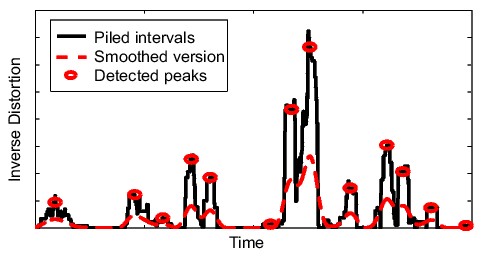
We deal with this by aggregating the extract a set of time indices
from the audio stream by aggregating the inverted distortion profiles
of the alignment paths to form a similarity profile over time. After
smoothing the similarity profile with a triangular averaging window,
we take the peaks from the resulting smoothed profile and use them
to represent the multiple paths overlaying that point in time. The
extracted time indices demarcate locations that bear resemblance to
other locations in the audio stream. This process is shown in Figure 2.
The reasoning behind this procedure can be understood by noting that
only some portions of the audio stream will have high similarity (i.e.
low distortion) to other portions. By focusing on the peaks of the
aggregated similarity profile, we restrict ourselves to finding those
locations that are most similar to other locations. Since every alignment
path covers only a small segment, the similarity profile will fluctuate
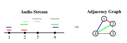
over time. This causes the audio stream to separate naturally into
multiple nodes corresponding to distinct patterns that can be joined
together in an adjacency graph as shown in Figure
3.
|
| Figure 2: Production of an adjacency graph
from alignment paths and extracted nodes. The audio stream
is shown as a timeline, while the alignment paths are shown
as pairs of colored lines at the same height above the timeline.
Node relations are captured by the graph on the right, with
edge weights given by the path similarities. |
|
| Figure 3: Production of an adjacency graph
from alignment paths and extracted nodes. The audio stream
is shown as a timeline, while the alignment paths are shown
as pairs of colored lines at the same height above the timeline.
Node relations are captured by the graph on the right, with
edge weights given by the path similarities. |
- Cluster Identification
The procedure we use to assign words to the clusters generated from
the previous section is relatively straightforward. For a given cluster,
C, a phonetic recognizer is used to transcribe the interval
underlying each node and convert it into a set of n-phones.
Likewise, the pronunciations for all words in a large baseform dictionary,
W, are converted into sets of n-phones. This process
reduces each node,  , and each
word, , and each
word,  , into sets of n-phone
sequences. By comparing the similarity of the words in the dictionary
to the nodes in C, the most likely candidate word common
to the cluster can be found. The hypothesized cluster identity is
given by , into sets of n-phone
sequences. By comparing the similarity of the words in the dictionary
to the nodes in C, the most likely candidate word common
to the cluster can be found. The hypothesized cluster identity is
given by
In this equation, we use the normalized intersection between the
sets and as a measure of similarity and aggregate this over all nodes
in the cluster for each word. We include the  factor in the denominator to normalize for the size of
and , so that longer/shorter words are not favored due to their
length. The factor of 2 in the numerator is included so that the overall
score ranges between 0 and 1. Using this similarity score, we can
easily generate an N-best list of word candidates for each
cluster.
factor in the denominator to normalize for the size of
and , so that longer/shorter words are not favored due to their
length. The factor of 2 in the numerator is included so that the overall
score ranges between 0 and 1. Using this similarity score, we can
easily generate an N-best list of word candidates for each
cluster.
Experiments and Results
The speech data used for our experiments is taken from a corpus of audio
lectures collected at MIT [2]. The entire corpus consists
of approximately 300 hours of lectures from a variety of academic courses
and seminars. The audio was recorded using an omni-directional microphone
in a classroom environment. In a previous paper, we described characteristics
of this lecture data and performed recognition and information retrieval
experiments [3]. Each lecture typically contains a
large amount of speech (from thirty minutes to an hour) from a single
person in an unchanging acoustic environment. On average, each lecture
contained only 800 unique words, with high usage of subject-specific words
and phrases. Each of the lectures used in our experiments was taken from
courses in computer science (CS), physics, and linear algebra.
| Computer Science |
| Cluster Size |
Common Word(s) |
Purity |
Hypothesis |
Score |
| 72 |
square root |
1.00 |
square |
0.23 |
| 40 |
procedure |
0.97 |
procedure |
0.34 |
| 21 |
combination |
1.00 |
commination |
0.43 |
| 19 |
computer |
1.00 |
computer |
0.63 |
| 17 |
primitive |
0.94 |
primitive |
0.12 |
| 14 |
definition |
1.00 |
definition |
0.29 |
| 12 |
parentheses |
1.00 |
prentice |
0.29 |
| 12 |
product |
0.83 |
prada |
0.65 |
| 10 |
operator |
0.80 |
operator |
0.37 |
| 10 |
and |
1.00 |
and |
0.29 |
|
| Linear Algebra |
| Cluster Size |
Common Word(s) |
Purity |
Hypothesis |
Score |
| 73 |
combination |
0.52 |
combination |
0.26 |
| 46 |
be |
0.24 |
woodby |
0.03 |
| 45 |
column |
1.00 |
column |
0.85 |
| 42 |
and |
0.64 |
manthe |
0.04 |
| 32 |
minus |
0.94 |
minus |
0.45 |
| 30 |
matrix |
0.97 |
matrix |
0.69 |
| 27 |
is |
0.56 |
get |
0.08 |
| 22 |
right hand side |
0.95 |
righthand |
0.46 |
| 14 |
picture |
1.00 |
picture |
0.88 |
| 11 |
one and |
1.00 |
wanna |
0.26 |
|
| Physics |
| Cluster Size |
Common Word(s) |
Purity |
Hypothesis |
Score |
| 21 |
is |
0.24 |
paced |
0.05 |
| 18 |
charge |
1.00 |
charge |
0.76 |
| 17 |
positively |
0.76 |
positively |
0.48 |
| 16 |
electricity |
1.00 |
electricity |
0.71 |
| 9 |
forces |
0.89 |
forces |
0.72 |
| 9 |
positive |
0.89 |
positive |
0.94 |
| 7 |
gravitational |
1.00 |
invitational |
0.61 |
| 6 |
times ten to |
1.00 |
tent |
0.57 |
| 6 |
distance |
0.83 |
distance |
0.51 |
| 5 |
gravity |
1.00 |
gravity |
0.44 |
|
Table 1: Ten largest clusters for
lectures in computer science, linear algebra, and physics. From
left to right, the columns list cluster size, the underlying common
reference word(s) for the cluster, the cluster purity (fraction
of nodes containing the common reference word(s)), the top cluster
identity hypothesis, and the hypothesis score. |
In Table 1 , we show example clusters from each
lecture ranked by size and include the results of the cluster identification
algorithm. At first glance, we found that the identification procedure
worked surprisingly well given that we did not use a unigram language
model to bias the baseform dictionary prior to search. We show individual
clusters rather than overall identification accuracy because we found
the types of errors made by the algorithm particularily enlightening.
The errors highlighted in blue originate
with the clustering component of our algorithm. The clusters erroneously
combine acoustically similar, but lexically dissimilar nodes consisting
of function word sequences, and word components. Examples include {"this
is", "misses", "which is"} and {"would be", "b", "see"}. The lexical disagreement
for these clusters can be seen in their purity scores, which measures
what fraction of the nodes contain the most common reference word(s) for
the cluster. An important observation we can make, however, is that the
scores for the hypothesized words are very low, indicating that we can
use the identification score as a metric for rejecting these types of
clusters.
The errors highlighted in purple and
pink can be attributed to limitations of the identification procedure.
Multi-word phrase clusters induce purple
errors, where the best matching single word in the dictionary only partially
covers the reference phone sequence. In the case of "right hand side"
and "square root", the algorithm finds one of the constituent words, but
for "times ten to", the best matching word is "tent", which occurs phonetically,
but not lexically, in the phrase.
Pink errors are characterized by single-word
clusters with relatively high purity. Upon examining the node phonetic
transcriptions, we concluded that the errors for these cases is due to
the inability of the phonological rules to account for the surface realization
of the word. Conspicuous examples are all present in the CS lecture, where
the lecturer consistently omits the "b" in "combination" and omits both
schwas in "parentheses". In the future, we may be able to mitigate these
errors by using more powerful phonological rules or by adopting a more
flexible search phase. It is interesting to note that almost all of these
errors occurred in the CS lecture, which suggests that their occurrence
may be dependent on speaking style.
Ongoing Research
In the future, we plan to improve upon the results we have presented
by iterating the word discovery process and by using phone lattices instead
of the top phone transcription during the cluster identification stage.
We can also incorporate lexical knowledge to help identify clusters by
using the word N-best lists for each cluster to find the set
of words that maximizes some joint probability of all words occurring
in a single document. Even without the cluster identification component,
we believe that our approach has many potential uses. In many tasks involving
the organization of large amounts of audio data, the core idea of pattern
discovery may be more suitable than a traditional speech recognizer because
it is completely language independent and requires no training data. The
unsupervised nature of the algorithm also makes it useful for improving
our understanding of how to learn directly from speech.
References:
[1] A. Park and J. Glass, Towards Unsupervised Pattern
Discovery in Speech. In Proc. IEEE Workshop on Automatic Speech Recognition
and Understanding, San Juan, Puerto Rico, December 2005.
[2] J. Glass, T. J. Hazen, L. Hetherington, and C.
Wang, Analysis and Processing of Lecture Audio Data: Preliminary investigations.
In Proc. HLT-NAACL 2004 Workshop on Interdisciplinary Approaches to
Speech Indexing and Retrieval, pp. 9--12, Boston, May 2004.
[3] A. Park, T. J. Hazen, and J. Glass, Automatic
processing of audio lectures for information retrieval: Vocabulary selection
and language modeling, In Proc. ICASSP , pp. I--497--450, Philadelphia,
2005. |

|