Research Abstracts - 2007

Introduction

A system’s ability to reason about its own decision making process is an important consideration in the design of real-time situated agents. This problem has been extensively studied in the literature, and is often referred to as meta reasoning, bounded rationality or the problem of computational resource constraints (Horvitz, 1988; Russell & Wefald, 1991; Zilberstein, 1993). The metalevel planning problem is usually modeled from a decision theoretic viewpoint where computational actions are taken to maximize the agent’s utility, generally computed as a function of the total expected time to completion. Recent work in metalevel planning exploits the properties of anytime algorithms (Boddy & Dean, 1994) and has focused on the problem of scheduling flexible planning components in order to achieve timely execution (Zilberstein & Russell, 1993).

One aspect of the problem that has not been addressed to the same extent is how the progress of the planner can be used to guide the planning process itself. If we view planning as a process of first solving sub-problems and then combining the sub-problems to form a complete plan, then the order that we choose to solve sub-problems has a significant effect on how quickly we converge to a good solution. As we will show, for repeated-planning problems where we expect to encounter multiple instances of planning problems in the same domains, it is possible to learn how previously solved sub-problems provide information about which sub-problem to solve next. Rather than having an algorithm decide a priori the order of solving subproblems using a fixed order (e.g., depth- or breath-first search), or by using a fixed cost function (e.g., A*-search), we will learn to use results of intermediate planning steps to guide the planning process..

Problem Formulation

We describe an approach to modelling metaplanning as a learned Markov decision process (MDP). We assume the existence of a decomposition of the planning problem into a series of sub-problems. The meta-planner learns a policy based on past experience of previous planning problems that either chooses another sub-problem to solve, or chooses to execute the best plan found so far. However, the size of an explicit MDP formulation of the meta-planning problem will grow exponentially with the number of sub-problems. We address this potential intractability using a policy class called the Decision Tree Meta Planner (DTMP), which allows us to represent the optimal policy compactly. The compactness is a result of pruning large portions of the plan space, leaving behind only those plan states that are expected to occur in the planning problem. Experimentally, we show that the DTMP is more compact than factored representations of the exact value function, allowing us to solve larger problems with negligible loss in performance.

The objective of our metalevel planner is to find and execute a minimum cost plan, where the total cost of the plan includes computation cost. The value of each sub-problem (i.e., the cost of using each sub-problem in the solution) is not known a priori but is drawn stochastically from a set of finite values according to some known distribution. An optimal meta-planning policy minimizes the expected cost with respect to the distribution of problem instances, where the cost is incurred by solving sub-problems and executing the best resulting plan.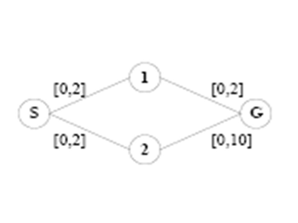

Figure 1. An extremely simple example planning problem. The objective is to compute the shortest path from S to G. In this case, the cost of each arc in an overall plan is drawn from an equally weighted Bernoulli distribution for costs [0; 2] or [0; 10].

The metaplanner knows the structure of the graph and that the distribution of possible costs of each arc is according to some Bernoulli distribution over [x; y]: note that the bottom-right arc has a much wider range of potential costs, and therefore a path through node 2 is much less likely to be the optimal solution. An optimal planner might solve this problem using dynamic programming, assigning a cost-to-go for each node by examining the cost of arcs in a particular order. If computation is free, then we can afford to consider all sub-problems with impunity and a dynamic programming strategy is reasonable. However, if computation costs are high, restricting the dynamic program to sub-problems only along the top path may be best. In particular, if the path through 1 is found to be low cost, then the additional computational effort of computing the cost through 2 may not be justified.

The MDP formulation for the meta-planning problem consists of a set of states, actions, rewards, and transitions. We consider finite horizon planning problems and do not discount. The states of the MDP are represented by the cross product of an information vector and the expected performance of the current best plan. The information vector is a vector whose length is equal to the number of sub-problems, where each element represents the current state of knowledge of the discretized cost the corresponding sub-problem. Unsolved sub-problems have are represented by an unknown, [?], cost indicator. The expected performance of the current plan is the expected cost that would be incurred if plan execution were to immediately take place. The number of actions is equal to the number of sub-problems plus 1. There are computational actions, which specifies and unsolved sub-problem to solve, and a single execution action, which executes the current best plan if one exists. The reward function consists separate time costs for computing sub-problems and executing plans. The transitions are learned from sample data. Solving the MDP results in a meta-planning policy specifying which sub-problems to solve, in what order to solve them, and when to execute the plan.

Note that this representation of the current plan state will grow exponentially with the number of sub-problems. Our naive formulation using the information vector means that the size of the resulting state space is O(|I|^|SP|) where |SP| is the number of sub-problems and |I| is the number of possible information values a sub-problem can take. This formulation clearly has an exponential dependence in the number of sub-problems and becomes computationally intractable quickly. For example for 16 sub-problems who can take on binary values, can have 43 million states.

Reducing the State Space

The reduction in state space can occur due to the realization that the MDP meta-planning problem formulation above yields a class of meta-planning policies which can naturally be interpreted in the form of a binary tree. The easiest way to see this is in the case of binary sub-problem costs. For instance starting at state s0 = [?; ?; ?; ?], the optimal policy may prescribe the action a0 = solvesp1. This results in a natural transition to either state s1 = [0; ?; ?; ?] or s2 = [2; ?; ?; ?], with no other possibility. This means that states which are reachable from s0 (e.g. [?; 0; ?; ?] or [?; 2; ?; ?]) other than s1 or s2 are automatically eliminated. Thus the first part of the policy can be represented as a tree, where the root node encodes both the state s0 and the optimal action a0 = solvesp1. The two branches of the tree correspond to the states resulting from the outcome of taking action a0. Since no plan state can be revisited, and no action can be taken twice, every meta-planning policy must be correspond to some policy tree.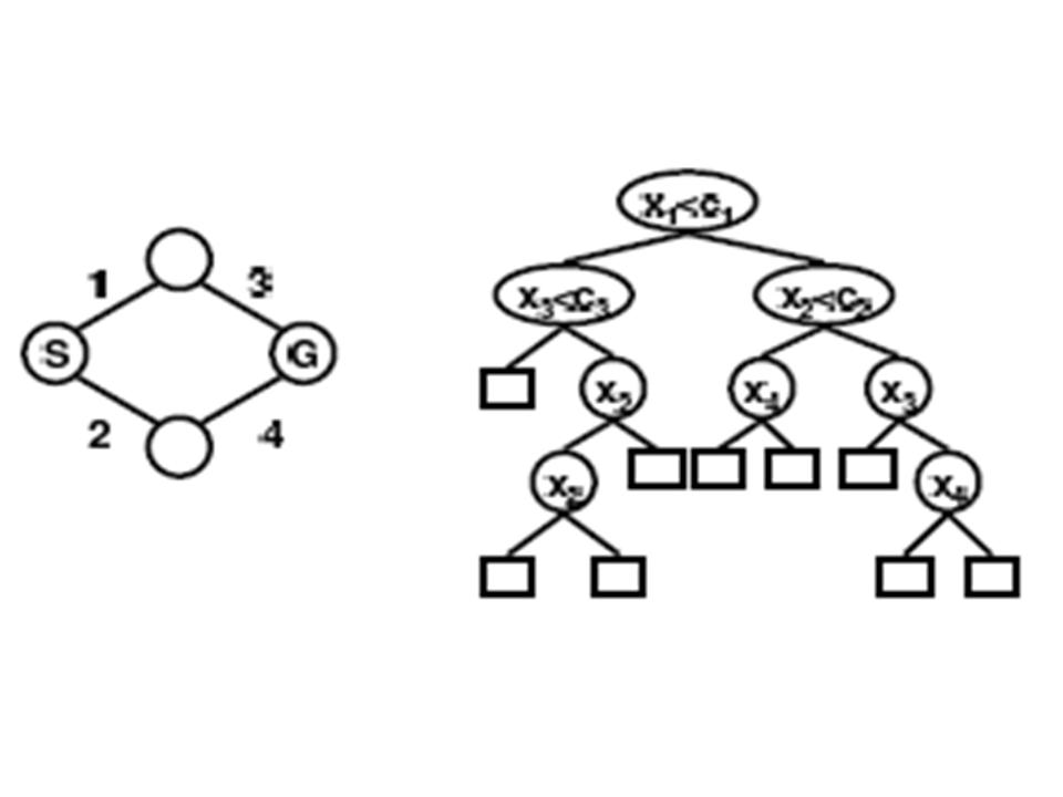

The figure above shows a small graph problem with 4 arcs and the corresponding policy tree on which to base the sequence sub-problems to conditionally solve. The first 3 internal nodes (circular nodes) of the tree are sub-problems to be solved, and each child represents an outcome in plan cost of the sub-problem. The square leaves of the tree represent the action to execute the current plan. The policy tree formulation provides one benefit, in that each child can represent a “split” in the plan cost, that is a range of posterior plan costs after the sub-problem is solved. For example, the left child is followed in the policy if the cost ci of parent xi is less than some threshold, otherwise the right child is followed. In this way, the policy tree does allow us to avoid discretizing the plan cost states as we had done in the conventional MDP. The policy tree can handle continuous plan values, and by virtue of the split selection, generates discretizations on its own.

Representing the policy as a tree does not automatically bring any computational savings; in the worst case, the policy tree will result in a structure that is exponential in the number of sub-problems with O(|I|^|SP|) nodes, leading to no savings compared to the previous state space formulation. However, a complete policy tree that stores the optimal action for every possible state will be unnecessarily large because it includes policy for states may have little or no consequence on generating good plans. For instance, the problem in figure 1 would require 43 states to completely represent it, but maintaining a policy for a state such as [0; 2; 0; 10] is unnecessary. In this case, the planner should never have computed the cost of the complete plan through both nodes 1 and 2 to reach this state. Discovering one of the lower, high-cost arcs should have been sufficient to guide the planner to complete the plan through node 1 and complete execution. Eliminating unnecessary states from the policy tree should result in a much more compact policy, where the size of the tree T, |T| << |I|^|SP| on average. In addition, we also reduce the action space by eliminating the need for the complete set of actions {A_compute} which included compute actions for each sub-problem. We now just have a single action acompute which solves the sub-problem given at the current state in the tree.

We now have a compact way of representing meta-planning policies, but arriving at them still requires solving the fullscale MDP. In order to circumvent this, we propose generating policy trees directly. One reasonable way to do this is to employ classification and regression tree learning to train a decision tree to act as an approximate meta-planning policy. We therefore collect training data.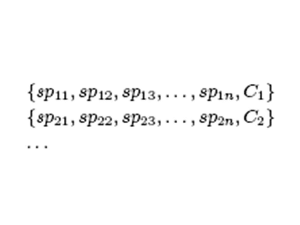

where each spij corresponds to the cost of using the solution to sub-problem i in sampled planning problem j (e.g., the cost of including an arc in a complete path, or the cost of using a sub-problem in a dynamic programming solution). Each sample j is labelled with the cost of the optimal executable plan (Cj). We then build the decision tree by splitting on sub-problem costs using a variance reduction heuristic standard for decision tree learning algorithms. The sub-problem placed at the root of the decision tree will be the sub-problem that, if solved, most reduces the variance of the expected plan costs provided in the training data after the split.

Results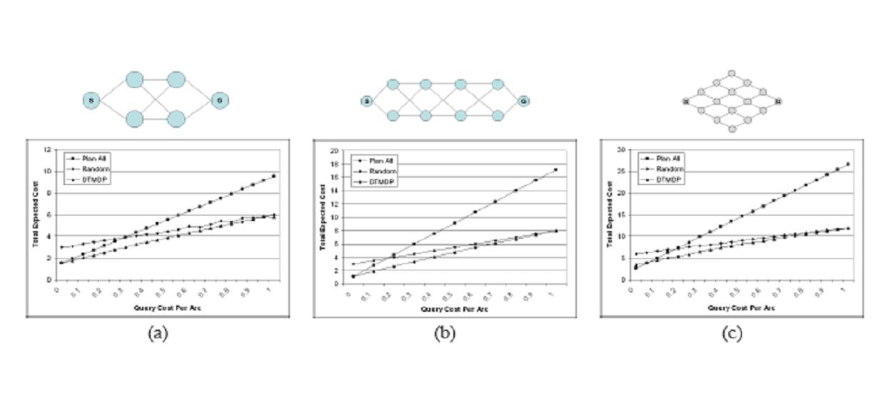

We tested the DTMP algorithm on several different planning domains, including shortest path type problems as in the graph examples as shown above as well as on mazes. We also tested it on a vehicle routing domain, where sub-problems consisted of determining the optimal routes for individual vehicles, which were combined to form a whole plan. In all problems the objective was to minimize the expected sum of computation and execution costs. In the graph examples above, we show, along with results from the DTMP algorithm, results for a standard plan to optimality algorithm, and a greedy algorithm, which plans sub-optimally, but quickly. The cost of computing each sub-problem, corresponding to determining the cost of an individual arc, is varied along the x-axis. The y-axis represents the expected total cost (the cost for computation plus the cost for execution) for each setting of the cost of computation, (the lower the better since we are minimizing cost). When computation costs are low, the plan to optimality planner does very well and the greedy algorithm performs poorly. When computation costs are high the optimal planner expends too much time solving sub-problems, and the greedy planner dominates. The DTMP solution is able to adapt to each case, transitioning from solving all sub-problems to planning greedily at the extremes. For intermediate values for the cost of computation, it is able to do better than both algorithms by selecting relevant sub-problems to solve and executing plans at the correct moments.

References:

[1] Author A. Lastname and Author B. Lastname. Title of the paper. In The Proceedings of the Conference, pp. 1--3, City, State, Country, Month 2004.

[1] M. Boddy and T. Dean. Decision-theoretic deliberations scheduling for problem solving in time-constrained environments. In Artificial Intelligence, 67(2), pp. 245--286, 1994.

[1] E. Horvitz. Reasoning under variying and uncertain resource costraints. In National Conference on Artificial Intelligenece (AAAI-88), pp. 111--116, 1988.

[1] S. Russell and E. Wefald. Do the right thing: Studies in limited rationality. The MIT Press. 1991.

[1] S. Zilberstein. Operational rationality through compilation of anytime algorithms. PhD dissertation. University of California at Berkeley, Department of Computer Science. 1993.

[1] S. Zilberstein and S. Russell. Anytime sensing planning and action: A practical model for robot control. In IJCAI , pp. 1402--1407. 1993.