Research Abstracts - 2007

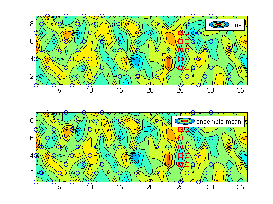
Introduction

Recent advances in numerical weather prediction (NWP) models have greatly improved the computational tractability of long-range prediction accuracy. However, the inherent sensitivity of these models to their initial conditions, due to its chaotic nature, has further increased the need for accurate and precise measurements of the environmental conditions.

Especially over the less frequently observed areas of the oceans, the initial conditions tend to be more inaccurate. Deploying an wide-area mobile observation network is likely to be costly, and measurements may produce different results in terms of improving forecast performance. These facts have led to the development of adaptive or targeted observation strategies where additional sensors are deployed to achieve the best performance according to some measures such as expected forecast error reduction and uncertainty reduction [1,2].

Our team developed an information-theoretic algorithm for selecting measurements in coarse scale [3,4]. However, it's a computationally intensive task to be done in fine resolution for real operation. Therefore, this research focuses on learning algorithms to use past experience in predicting good routes to travel between measurements choosen by above algorithm, which will gives us a quick answer, once the model is learned [4].

Models of Weather Prediction

While there exist large-scale realistic models of weather prediction such as the Navy's Coupled Ocean Atmosphere Prediction System (COAMPS), our attention will be first restricted to reduced models in order to allow computationally tractable experiments with different adaptive measurement strategies. The Lorenz-2003 model address multi-scale feature of the weather dynamics in addition to the basic aspects of the weather motion such as energy dissipation, advection, and external forcing [5].

State Estimation

A standard approach to state estimation and prediction is to use a Monte Carlo (ensemble) approximation to the extended Kalman Filter, in which each ensemble member presents an initial state estimate of the weather system. These ensembles are propagated (for a set forecast time) through the underlying weather dynamics and the estimate (i.e., the mean value of these ensembles) is refined by measurements (i.e., updates) that are available through the sensor network. The particular approximation used in this work is the sequential ensemble square root filter (EnSRF) [6].

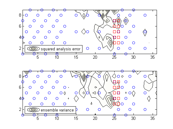
Figure 1 (left) True vs. Estimated State (right) Performance anaylsis

The rountine observations spots are represented by blue circles in the above figure, where observations are taken every 6hrs. We can see the uncertainty around the region where the blue circles are sparsely located. For the purposes of forecast error, we are typically interested in improving the forecast accuracy for some small region such as the coast of California, rather than the entire Pacific. A verification region is specified as the red squares in Figure. Our goal is therefore to choose measurements to minimize the forecast error at the verification region at some forecast time (eg. 2~4 days after taking measurements)

Trajectory Learning

The problem of learning a model that minimizes the predicted forecast error is that of reinforcement learning, in which an agent takes actions and receives some reward signal. If our set of actions is chosen to be a class of paths through space, such as polynomial splines interpolating the target points, then the policy attempts to choose the best spline to minimize our expected forecast error. The policy does not have access to the current weather state but only the current estimate of the weather given by the EnSRF. The learner therefore computes the policy that chooses actions based on the current estimate given by the mean and covariance of the ensemble.

The SVM is a good choice to learn our policy for two reasons: firstly, the SVM allows us to learn a classifier over the continuous state space. Secondly, the SVM is generally an efficient learner of large input spaces with a small number of samples; the SVM uses a weighted distance function to perform classification by projecting each instance to a high-dimensional, non-linear space in which the inputs are linearly separable according to their class label [7]. Finding an appropriate ``kernel'' or set of features for this type of problem is one of the challenges of using a learned classifier for predicting good trajectories.

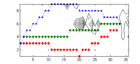
Figure 2 Example trajectories

Initially, we have restricted the learner to a limited set of 5 actions or candidate trajectories, although this constraint will be relaxed in future work. All candidate trajectories started from the same mid-point of the left side of the region and ended at the same mid-point of the right side of the region. Three examples of the five trajectories are shown in the above figure; the trajectories were chosen to be maximally distinct through the area of sparse routine observations in the centre of the region.

From the initial conditions, the model and ensemble were propagated for each trajectory. During this propagation, routine observations were taken every 5 time units and then a forecast was generated by propagating the ensemble for time equivalent to 2 and 4 days, without taking additional observations. The forecast error was then calculated by the difference between the ensemble estimate and the true value of the variables of the verification region. Each initial condition was labelled with the trajectory that minimized the resultant forecast error.

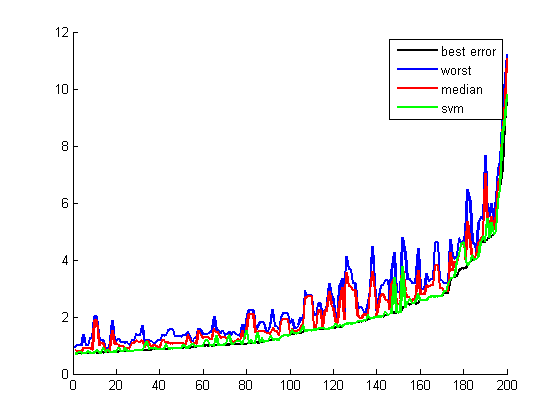
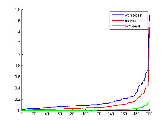
Figure 3 (left) Forecast error (right) Forecast error loss

The left figure above shows the forecast error of best, median, worst and SVM trajectory for the 200 most difficult (highest forecast error) initial conditions in terms of the forecast error in the verification region. Notice that the forecast error of the SVM trajectory tracks the best trajectory relatively closely, indicating good performance. The right above figure is an explicit comparison between the worst, median and SVM trajectories compared to the best trajectory for the same 200 most difficult training instances. Again, the SVM has relatively little loss measured by the difference between the forecast error of the SVM and the forecast error of the best trajectory) for many of these difficult cases. In training the learner, two different kernels were tested: a polynomial kernel and a radial basis function (RBF) kernel. Using cross-validation and a standard parameter search method to identify the best kernel fit and size, a surprising result was that a low-order polynomial kernel resulted in the most accurate prediction of good trajectories. However, further investigation is needed.

The spatio-temporal character of the data and chaotic behavior of the weather model results in a challenging adaptive observation problem in the weather domain. In the future, we plan to extend these results using the Navy's Coupled Ocean Atmosphere Prediction System (COAMPS), a full-scale regional weather research and forecasting model.

References:

[1] http://www.aoc.noaa.gov/article_winterstorm.htm, Available online (last accessed June 2005)

[2] Morss, R., Emanuel, K., Snyder, C. Idealized adaptive observation strategies for improving numerical weather prediction. Journal of the Atmospheric Sciences), 2001

[3] Choi, H.L., How, J., Hansen, J. Ensemble-based adaptive targeting of mobile sensor networks. In Proc. of the American Control Conference (ACC), To appear. 2007

[4] Nicholas Roy, Hanlim Choi, Daniel Gombos, Jonathan How, Jim Hansen and Sooho Park. Adaptive Observation Strategies for Forecast Error Minimization. Dynamic Data Driven Application Systems (DDDAS) Workshop on International Conference on Computational Science (ICCS), to appear, Beijing, China, 2007

[5] Lorenz, E.N., Emanuel, K.A. Optimal sites for supplementary weather observations: Simulation with a small model. Journal of the Atmospheric Sciences, pp. 399--414, 1998

[6] Evensen, G., van Leeuwen, P. Assimilation of altimeter data for the agulhas current using the ensemble kalman filter with a quasigeostrophic model. Monthly Weather Review pp. 85--96, 1996

[7] Cristianini, N., Shawe-Taylor, J. An Introduction to Support Vector Machines. Cambridge University Press, Cambridge, UK, 2000