MIT CSAIL Research Abstracts

CSAIL Publications and Digital Archive header

Research Abstracts Home

CSAIL Digital Archive

Research Activities

CSAIL Home

horizontal line

Research Abstracts - 2007
horizontal line

horizontal line

Table 2 shows the average total execution time on 5.5 hours of data for the three methods. EBW performs more than 5 times faster than BIC and 3 times faster than CUSUM. At each new hypothesized boundary within an observation sequence, BIC re-estimates model parameters. However, EBW and CUSUM only estimate model parameters once within an observation sequence. Yet, CUSUM computes the inverse covariance and determinant in the likelihood formulation, and is thus slower than EBW which computes variances.

Audio Segmentation and Classification using Extended Baum-Welch Transformations

Tara N. Sainath & Victor Zue

Introduction

Audio steams, such as broadcast news or meeting recordings, contain audio from a wide variety of sources, including speech, music, coughing, laughter, etc. Segmentation and classification have become important tools to describe an audio scene that contains a variety of acoustic events. In our work, we use the Extended Baum-Welch (EBW) transformations [1] to develop novel segmentation and classification approaches. Specifically, in [2] we show that our segmentation algorithm offers improvements over two baseline methods, namely the Bayesian Information Criterion (BIC) [3] and Cumulative Sum (CUSUM) [4] methods. In addition, in [5] we use these transformations to develop a novel audio classification algorithm, which is able to outperform both the Gaussian Mixture Model (GMM) Likelihood and Support Vector Machine (SVM) classification techniques.

Extended Baum-Welch Transformations

The EBW procedure involves continuous transformations that can be described as follows. Assume that data $X= (x_{1}, ...x_{n})$ , from frames 1 to n, is drawn from a mixture of M Gaussians, with each component is described by the following mean, variance and weight parameters $\lambda_j = \{\mu_j,\sigma_j, w_j\}$ . Let us define the probability of frame $x_i \in X$ given model $\lambda_j$ as $z_{ij} =p(x_i\vert\lambda_j)$ and let $F({z_{ij}})$ be some objective function over ${z_{ij}}$ . In our work, we consider $F_{1,n}(z_{ij})$ to be the log-likelihood over the data as $F_{1,n}(z_{ij})=p(X\vert\lambda_j)=\sum_{t=1}^n \log \sum_{k=1}^M w_k z_{tk}$ . Given this function and initial model parameters $\lambda_j$ , the EBW provide formulas to re-estimate model parameters $\lambda_j(D) = \{\mu_j(D),\sigma_j(D)\}$ . Here D is a large constant chosen such that value of the objective function increases with each iteration, that is $F_{1,n}(\hat{z}_{ij}) >F_{1,n}(z_{ij})$ . Using EBW transformations such that $\lambda_j \rightarrow \hat{\lambda}_j(D)$ and $\{z_{ij} \} \rightarrow {\{\hat{z}_{ij}} \}$ , [1] derives a linearization formula between $F_{1,n}({\hat{z}_{ij}} )$ and $F_{1,n}(z_{ij})$ for large D as:

$\begin{displaymath} F_{1,n}({\hat{z}_{ij}})- F_{1,n}(z_{ij}) = T_{1,n}^{\lambda_j}/D +o(1/D) \end{displaymath}$

(1)

Here $T_{1,n}^{\lambda_j}$ measures the gradient required to adapt initial model $\lambda_j$ to data X , or equivalently how well the data is explained by the initial model $\lambda_j$ . [1] also derives a closed form expression for $T_{1,n}^{\lambda_j}$ . In our work, we explore using both sides of Equation 1, namely T and the difference in objective functions F , to develop our EBW segmentation and classification techniques.

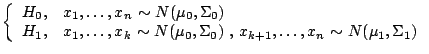
Segmentation via EBW Transformations

The goal of a segmentation algorithm is to divide an audio segment into homogeneous regions. Given observations $(x_1, \ldots ,x_n)$ , the EBW hypothesis tests for a change at point k is as follows: $\left\{ \begin{array}{lll} H_0, & \hbox{$x_1, \ldots ,x_n$\ $\sim$\ $ N(\mu_0... ...\ , $ x_{k+1}, \ldots ,x_n$\ $\sim$\ $ N(\mu_1, \Sigma_1)$} \end{array}\right.$

Using the above two hypothesis, our segmentation criterion becomes:

$\begin{displaymath} \hat{k}=\arg \min_{k} \{T_{k+1,n}^{\lambda_1} + T_{1,k}^{\lambda_0} - T_{1,n}^{\lambda_0}\} \leq \epsilon \end{displaymath}$

(2)

Intuitively this means that we detect a change at point $\hat{k}$ if ( $x_1, \ldots ,x_{k}$ ) is explained better by $\lambda_0$ (i.e. $T_{1,k}^{\lambda_0}$ ) and ( $x_{k+1}, \ldots ,x_{n}$ ) is explained better by $\lambda_1$ (i.e. $T_{k+1,n}^{\lambda_1}$ ), rather than the entire sequence being explained by $\lambda_0$ (i.e. $T_{1,n}^{\lambda_0}$ ). The better the data is explained by a specific set of models, the smaller T is, so we look for the change point k which produces the minimum T and compare this to an empirically found threshold $\epsilon$ . Since many unsupervised segmentation algorithms suffer from missed landmarks and oversegmentation problem, we also explore additional landmark refinement and merge stages discussed in [2], to alleviate these problems.

Classification via EBW Transformations

Given a set of class models $\Lambda=\{\lambda_1, \lambda_2, \ldots, \lambda_K\}$ , the goal of classification is to categorize an ensemble of input frames $X=\{x_1,\ldots,x_n\}$ , where $x_i \in R^d$ , as belonging to one of these models. The best model $\lambda_j \in \Lambda$ is the one which explains the data best, and is defined as one for which $T_{1,n}^{\lambda_j}$ is smallest. We will refer to this classifier as EBW-T and accordingly our decision rule for the best class can be written as:

$\begin{displaymath}\lambda^* = arg \min_{j} T_{1,n}^{\lambda_j} \end{displaymath}$

(3)

We can also use the formula given in the right side of Equation 1 for classification. Here D is a constant chosen in the EBW re-estimation formulas $\lambda_j(D) = \{\mu_k(D),\sigma_j(D)\}$ . Thus, given an input sample X, the best class model $\lambda_j$ is the one which has the smallest increase in likelihood given the update model $F_{1,n}({\hat{z}_{ij}(D)})$ relative to the likelihood given the initial model $F_{1,n}(z_{ij})$ . Using this EBW-F classifier, the decision rule for the best model is:

$\begin{displaymath} \lambda^*= arg \min_{j} \left\{ F_{1,n}({\hat{z}_{ij}(D)})- F_{1,n}(z_{ij}) \right \} \times D \end{displaymath}$

(4)

In [6], Valtchev et.al shows that using a phone-specific D instead of a global value allows for better re-estimated phoneme models using the EBW transformations. Similarly, in [5] we show that different classes prefer a specific D value when estimating the updated model $\lambda_j(D)$ . Since each class has a different preferred D value, we construct a feature vector from scores obtained from evaluating $\left\{F_{1,n}({\hat{z}_{ij}(D)})- F_{1,n}(z_{ij}) \right \} \times D$ for different D, and train an SVM classifier from the transformed feature space. We will refer to this classifier as the EBW-SVM classifier.

Experiments

We perform segmentation experiments using the Computers in the Human Interaction Loop (CHIL) Isolated Acoustic Event data set [7]. This data set contains isolated acoustic events from 15 different classes, including knocks, doors opening/closing, applause, laughter, etc. The set is divided into 3 sessions, with 10 participants per session. In total, there are over 6000 change points per session, which are annotated manually by the University Polytechnic of Catalonia (UPC). Our segmentation experiments use 19 dimension Mel-Frequency Cepstral Coefficients (MFCCs) while our classification experiments compare both MFCCs and MFCCs plus perceptual features, including short-time energy, zero crossing rate, subband energy spectral flux.

Results

To evaluate our segmentation algorithms, we compute the F-measure, which measures the tradeoff between precision and recall. Table 1 shows the evaluation metric scores for the CUSUM, BIC and EBW algorithms, the latter with and without the refinement and merge stages. Note that the BIC implementation discussed here also includes a similar refinement and merge stage. One reason that EBW outperforms CUSUM is that each term T in EBWSeg captures the difference between the likelihood of a data given the initial model and the likelihood with a model estimated from the entire data sequence, while CUSUM just calculates the former. The EBW with the refinement and merge stage is able to outperform BIC. One theory is that the objective of an EBW-hypothesized test is to minimize detection time for a given false alarm rate, which closely matches the goal of segmentation.

CHIL Data Segmentation Results
	Session 1			Session 2			Session 3
	Precision	Recall	F-measure	Precision	Recall	F-measure	Precision	Recall	F-measure
EBWSeg, ref. & merge	0.87	0.83	0.85	0.88	0.82	0.85	0.88	0.83	0.85
EBWSeg	0.84	0.80	0.82	0.86	0.80	0.83	0.86	0.82	0.83
BIC	0.84	0.79	0.81	0.85	0.81	0.83	0.87	0.81	0.83
CUSUM	0.76	0.76	0.76	0.78	0.76	0.77	0.79	0.77	0.78

Table 1: Segmentation Results for EBW, CUSUM and BIC

Segmentation Algorithm	Average Total Execution Time (hrs)
EBWSeg, ref. & merge	0.42
BIC	2.25
CUSUM	1.43

Table 2: Average Total Execution Time of Segmentation Algorithms

Table 3 shows the classification results for the baseline and EBW classifiers using both MFCC and MFCC+Perceptual features. The EBW-T and GMM offer comparable performance. However, when we are able to control how fast we update our model using EBW-F classifier, we outperform both EBW-T and GMM for both feature sets. Again we see that using EBW to re-estimate trained models with the current data sequence being classified offers improvements over the standard GMM likelihood approach. As expected, the SVM outperforms the GMM and EBW models on all feature sets. However, transforming the feature space using the scores of EBW-F classifiers for different D offers improvements over the baseline SVM.

Classifier	MFCCs	MFCCs+Perc
GMM Baseline	88.91	91.88
SVM Baseline	92.43	93.04
EBW-T	89.82	91.19
EBW-F	90.27	93.04
EBW-SVM	92.64	94.78

Table 3: Classification Results for EBW and Baseline Classifiers

Ongoing Research

Audio segmentation and classification are often used as preprocessing step in speech recognition to separate an audio stream into homogeneous regions where each region can be handled in a different manner. We are currently looking to apply these EBW techniques for multilevel preprocessing, include speech/non-speech and broad phonetic class detection, to improve robustness of speech recognition systems.

Acknowledgements

This reseach is sponsored by the T-Party Project, a joint research program between MIT and Quanta Computer Inc., Taiwan. We would also like to thank Dimitri Kanevsky and Giridharan Iyengar of IBM for their contributions and inputs to this work.

References

[1] D. Kanevsky. Extended Baum Transformations for General Functions. In Proc. ICASSP, 2004.

[2] T.N. Sainath, D. Kanevsky, and G. Iyengar. Unsupervised Audio Segmentation using EBW Transformations. To Appear in Proc. ICASSP, 2007.

[3] S. Chen and P. Gopalakrishnan. Speaker, Environment and Channel Change Detection and Clustering via The Bayesian Information Criterion. In Proc. Broadcast News Trans. and Under. Workshop , February 1998, pp. 127–132.

[4] M. Omar, U. Chauduri, and G. Ramaswamy. Blind Change Detection for Audio Segmentation. In Proc. ICASSP, 2005.

[5] T.N. Sainath, V. Zue, and D. Kanevsky. Audio Classification using EBW Transformations. Submitted to ICSLP, 2007.

[6] V. Valtchev, J.J. Odell, P.C. Woodland, and S.J. Young. MMIE Training of Large Vocabulary Speech Recognition Systems. In Speech Communication,, vol. 22, no. 303-314, 1997.

[7] A. Waibel et al., CHIL: Computers in the Human Interaction Loop. In WIAMIS, 2004.

Computer Science and Artificial Intelligence Laboratory (CSAIL)
The Stata Center, Building 32 - 32 Vassar Street - Cambridge, MA 02139 - USA
tel:+1-617-253-0073 - publications@csail.mit.edu