Introduction

In recent years, several methods have been proposed that permit the usage of global incident lighting in real-time rendering [1,2]. These approaches represent the incident radiance in spherical harmonics (SH). They, however, assume distant lighting. As a result, they are incapable of rendering scenes with close-range lighting effects without visual error.

We propose to compute a first-order Taylor expansion of the spherical harmonic coefficients around a lighting sample point. We show how the gradient of the incident radiance (represented in SH) can be computed for little additional cost compared to the coefficients alone. A semi-analytical formula is introduced to calculate this gradient at run-time. The incident radiance can now be extrapolated to different positions around the original sample location. In case of multiple samples, the interpolation quality is greatly improved, thus requiring less samples. Extrapolation/interpolation can be easily performed in a vertex shader on the GPU.

Figure 1: Head model moved underneath a local emitter from left to right. The incident lighting is only sampled once at the center of the head (middle image).

Approach

Given incident radiance at a point , we first project it into spherical harmonics yielding a coefficient vector . This vector of coefficients is usually reused for every point on the object that is to be displayed --- effectively moving the lighting to infinity. In contrast to this, we want to estimate what the incident radiance is at some point , where is the difference vector between the sample point and the current point , i.e., we want to estimate the coefficient vector .

To this end, we compute the gradient of incident lighting and use it to estimate the coefficients . The use of spherical harmonics, allows us to directly compute the gradient:

Here the y_i() are the spherical harmonic basis functions, and x is a point on a visible surface, n(x) is the normal, and s is the vector to the point x. As it turns out, this gradient can be expressed analytically and is cheap to evaluate.

At run-time, we estimate local lighting coefficients at every vertex of the object. The additional run-time cost is almost negligible. It only involves a simple dot-product and an addition, since the gradient only needs to be computed once when the incident lighting is sampled.

Results

The strength of the gradient method can be illustrated by moving an object below a small and local area light, see Figure 1. In this example, we compute the original incident lighting sample and the gradient only once at the center of the head in the middle image. We then move the head from left to right underneath the light. Shading is computed with our gradient method based on the single sample. Shading responds correctly to the change of location.

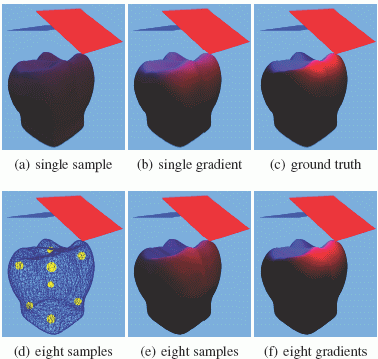
In Figure 2, a tooth model is illuminated by partially overlapping emitters. Different renderings compare extrapolation of a single sample against interpolation of eight samples. Rendering (b) uses a single sample with a gradient. It does similarly well as eight samples without gradients (see (e)). The only noticeable difference is the top of the tooth. Here visibility changes should make it mainly blueish, but the extrapolated single sample is purple. Interpolation of eight samples with gradients (f) produces virtually the same result as the reference image.

Figure 2: Comparison of a single sample versus multiple samples and gradients versus no gradients: (a) A single sample without gradient, (b) A single sample with gradient, (c) Reference model, (d) Eight sample locations, (e) Interpolation of eight samples without gradient, (f) Interpolation of eight samples using the gradients.

In our experience, a single sample using the gradient is often sufficient. Only for very nearby emitters --- where "nearby" means closer than the distance from the sample position to the object's bounding box (empirically determined) --- we have found that one needs multiple samples. In these cases the 1/r^2 falloff is very important and cannot be modeled by our first-order approximation.

Research Support

This research was supported by a NSF CISE Research Infrastructure Award (EIA-9802220), a DAAD (German Academic Exchange) and a DFG (German Research Foundadation) Post-Doc fellowship.

References

[1] P.-P. Sloan, J. Kautz, J. Snyder. Precomputed Radiance Transfer for Real-Time Rendering in Dynamic, Low-Frequency Lighting Environments. In ACM Transactions on Graphics, 21(3), pp. 527--536, July 2002.

[2] P.-P. Sloan, J. Hall, J. Hart, J. Snyder. Clustered Principal Components for Precomputed Radiance Transfer. In ACM Transactions on Graphics, 22(3), pp. 382--391, August 2003.